[HAI5016] Week 2: The Data Scientist toolkit

This week, we will equip ourselves with the essential tools for data science.

Disclaimer: This blog provides instructions and resources for the workshop part of my lectures. It is not a replacement for attending class; it may not include some critical steps and the foundational background of the techniques and methodologies used. The information may become outdated over time as I do not update the instructions after class.

1. Installation

In the first part we will install and configure:

• Miniconda (Python)
• Visual Studio Code
• Git

These installations will form the foundation of your workflow, making it easier to manage environments and work with data.

---

1.1 Miniconda (Python)

Miniconda is a lightweight Python distribution that comes with Conda for managing packages and environments. You can download it from the Miniconda official site. Follow the installation instructions based on your operating system:

On windows 10 & 11 (x64)

1. Download and install Miniconda using the following command in Command Prompt:

   curl https://repo.anaconda.com/miniconda/Miniconda3-latest-Windows-x86_64.exe -o miniconda.exe
   start /wait "" .\miniconda.exe /S
   del miniconda.exe
   

2. Set your PATH environment variables:

   setx PATH "%PATH%;%USERPROFILE%\miniconda3;%USERPROFILE%\miniconda3\Scripts;%USERPROFILE%\miniconda3\condabin"
   

To use the conda command, use the terminal in VSCode (when a conda environment is activated) or use the newly installed Anaconda Prompt.

On MacOS (Apple Silicon ARM)

1. Install Miniconda with the following commands:

   mkdir -p ~/miniconda3
   curl https://repo.anaconda.com/miniconda/Miniconda3-latest-MacOSX-arm64.sh -o ~/miniconda3/miniconda.sh
   bash ~/miniconda3/miniconda.sh -b -u -p ~/miniconda3
   rm ~/miniconda3/miniconda.sh
   

2. Initialize Miniconda for your shell (bash or zsh):

   ~/miniconda3/bin/conda init bash
   ~/miniconda3/bin/conda init zsh
   

---

1.2 Visual Studio Code

Visual Studio Code is the code editor of choice during this class due to its extensive integration with Python, Jupyter, Pandas and of course Copilot. Download the latest version at

• Download VS Code

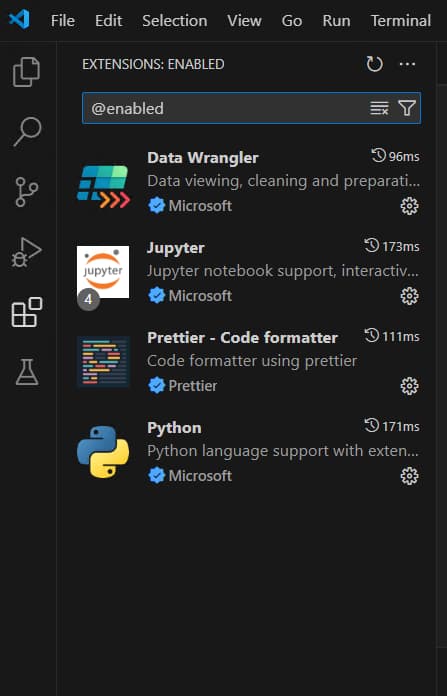
Essential Extensions for VS Code:

After opening VS code, open the extensions pane and click the ‘install’ button for the following extensions:

1. Python - Installs Pylance and the Python debugger.
2. Jupyter - Work with Jupyter Notebooks in VS Code.
3. Prettier - Code formatting to keep your code neat.
4. Data Wrangler - Interact with tabular data directly in VS Code.

1.3 Git

Git is a version control tool essential for tracking changes in your code and collaborating with others.

Git for windows

1. Download Git from the official site: Download Git for Windows.

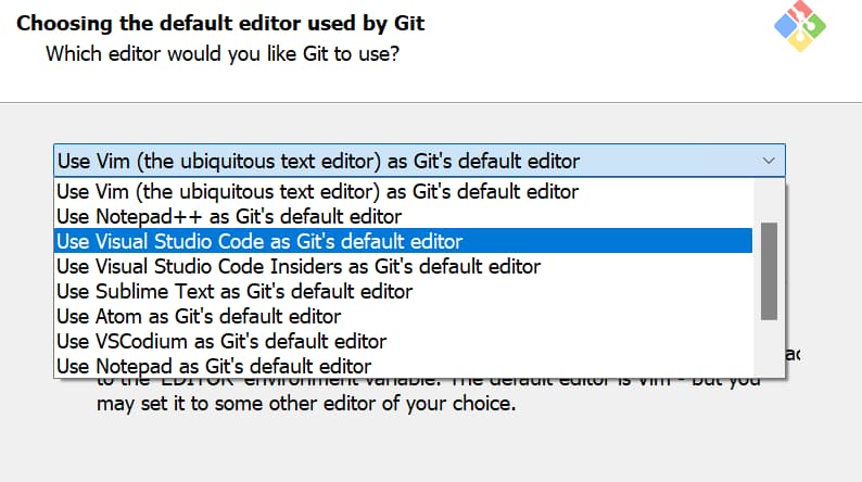
2. Run the installation. You can basically proceed with all the suggested settings, but I recommend you to select ‘Visual Studio Code’ as the default editor for git during set-up.

   

Git for MacOS

1. Check if Git is already installed by typing the following in the terminal:

   git --version
   

   On the latest versions of macOS, if Git is not installed, checking the Git version will trigger an installation prompt. By clicking ‘Install,’ macOS will automatically install the Xcode development tools along with Git, allowing you to skip steps 2 and 3 below.

2. If Git is not installed, first install Homebrew:

   /bin/bash -c "$(curl -fsSL https://raw.githubusercontent.com/Homebrew/install/HEAD/install.sh)"
   

3. Then, install Git:

   brew install git
   

Set Git Global Variables

Replace the placeholders with your own details.

   git config --global user.name "Handsome Professor" 
   git config --global user.email "prof@sky.com"

---

2. Setting Up Your Python Project

Now that we have installed the necessary tools, let’s practice by setting up a Python project from scratch. This part includes creating a virtual environment, writing Python code, and running it in VS Code. Let’s call our project HAI5016.

---

2.1 Creating a Virtual Environment

To isolate your project dependencies and avoid conflicts, we will create a virtual environment for your data project using Conda. We are going to call the virtual environment haienv, use Python 3.12 as a base and pre-install the python packages Pandas and Jupyter

1. Open the terminal on MacOS or Anaconda Command Prompt on Windows and run the following command to create an environment:

   conda create -n haienv python=3.12 pandas jupyter
   

2. Then, activate the newly created environment:

   conda activate haienv
   

This environment will contain Python, Pandas, Jupyter, for data analysis.

---

2.2 Creating a Project Folder

1. Create a folder on your PC in a convenient location to store your project files. Name this folder HAI5016.

2. Open this folder in Visual Studio Code using File > Open Folder.

---

2.3 Writing The First Python Script

1. From the VS Code File Explorer, you can use the New File icon to create a python file named helloworld.py.

2. Add the following code to your helloworld.py file:

   msg = "Hello World"
   print(msg)
   

3. Make sure to activate and select our ‘haienv’ virtual environment as the Python interpreter for VSCode.

---

2.4 (down)Loading our data

1. From the VS Code File Explorer, use the New File icon to create a new python file named download_data.py.

2. Type the following code:

   # Import the packages os and urllib.request
   import os
   import urllib.request
   
   # Create a directory in our project folder if it doesn't exist
   os.makedirs('titanic-data', exist_ok=True)
   
   # Set the source URL and destination path
   download_url = 'https://hbiostat.org/data/repo/titanic3.csv'
   file_path = 'titanic-data/titanic3.csv'
   
   # Download the file if it doesn't exist
   if not os.path.exists(file_path):
      urllib.request.urlretrieve(download_url, file_path)
   

Congratulations. If this went well, there should be a new folder in your project called titanic-data that contains the file titanic3.csv.

---

3 More Python - but in a Notebook

Let’s create a Jupyter Notebook:

1. Run the New Jupyter Notebook command from the Command Palette (Ctrl+Shift+P) or by creating a new .ipynb file in your project folder like you did before with the .py files.

2. Click on the kernel picker in the top right and select our virtual environment ‘haienv’

3. Save the notebook as titanic.ipynb by pressing crtl+s or cmd+s

4. In the new cell, type the same code as in our first Python script:

   msg = "Hello World"
   print(msg)
   

5. Hit Shift+Enter to run the currently selected cell and insert a new cell immediately below.

---

3.1 Load our data into a Dataframe

Let’s begin our Notebook journey by importing the Pandas and NumPy libraries, two common libraries used for manipulating data.

1. Copy and paste the following code into the first cell

   import pandas as pd
   import numpy as np
   

   And hit Shift+Enter to see if the libraries load successfully.

2. Then, let’s load the titanic data into the memory:

   data = pd.read_csv('titanic-data/titanic3.csv')
   

3. Let’s see what the data looks like by showing the top 5 records in our dataframe:

   data.head()
   

4. Let’s get an overview of the columns and their data types:

   data.dtypes
   

5. Explore the Variables and View data buttons that appeared in the editor.

6. Let’s replace the ‘?’ with missing data markers:

   data.replace('?', np.nan, inplace= True)
   data = data.astype({"age": np.float64, "fare": np.float64})
   

7. Let’s add a markdown cell to our Notebook with the meaning of several column names, so that we won’t have to look it up another time.

---

3.2 Visualize our data

With our data loaded into a dataframe, let’s use seaborn and matplotlib to view how certain columns of the dataset relate to survivability.

1. Load the seaborn and matplotlib packages into the memory:

   import seaborn as sns
   import matplotlib.pyplot as plt
   

2. Then, let’s write some code to visualize our data:

   fig, axs = plt.subplots(ncols=5, figsize=(30,5))
   sns.violinplot(x="survived", y="age", hue="sex", data=data, ax=axs[0])
   sns.pointplot(x="sibsp", y="survived", hue="sex", data=data, ax=axs[1])
   sns.pointplot(x="parch", y="survived", hue="sex", data=data, ax=axs[2])
   sns.pointplot(x="pclass", y="survived", hue="sex", data=data, ax=axs[3])
   sns.violinplot(x="survived", y="fare", hue="sex", data=data, ax=axs[4])
   

   ---

3.3 Calculate correlations

Visually, we may see some potential in the relationships between survival and the other variables of the data. With the pandas package it’s also possible to use pandas to calculate correlations, but to do so, all the variables used need to be numeric for the correlation calculation. Currently, sex is stored as a string. To convert those string values to integers, let’s do the following:

1. Check the values with data['sex']

2. Map the textual values with integers:

   data.replace({'male': 1, 'female': 0}, inplace=True)
   

3. Ceck the values again with data['sex']. The sex column should now consist of integers instead of strings.

4. Now we can correlate the relationship between all the variables and survival:

   data.corr(numeric_only=True).abs()[["survived"]]
   

5. Which variables seem to have a high correlation to survival and which ones seem to have little?

Let’s say we think that having relatives is related survivability. Then we could group sibsp and parch into a new column called “relatives” to see whether the combination of them has a higher correlation to survivability.

To do this, you will check if for a given passenger, the number of sibsp and parch is greater than 0 and, if so, you can then say that they had a relative on board:

   data['relatives'] = data.apply (lambda row: int((row['sibsp'] + row['parch']) > 0), axis=1)
   data.corr(numeric_only=True).abs()[["survived"]]

---

Sources and more

Here are some additional resources to help you get more familiar with the tools:

• VS Code Data Science Tutorial
• VS Code Tips & Tricks
• 10 essential VS Code tips & tricks for greater productivity

---